2005 to 2022 Local Authority Greenhouse Gas Emissions Dataset

This dataset includes territorial emissions, CO2 emissions within the scope of influence of local authorities, mid-year populations, and area sizes for the emissions of each greenhouse gas in each local authority greenhouse gas sub-sector in the UK from 2005-2022. Some rows are missing data for the Country Code, Region Code, Second Tier Authority, Mid-year Population, and Area columns. This dataset is from the UK government and the data was collected by the Department for Energy Security and Net Zero National Statistics of energy consumption for local authority areas and the UK National Atmospheric Emissions Inventory in the UK’s annual inventory of greenhouse gas emissions.

UK Regions GeoJSON

This document includes the coordinates for the borders of the twelve UK regions. This document is from Kaggle and was used to generate geospatial visualizations.

Tools

• Microsoft Excel: To store the dataset.
• Python and Jupyter Notebooks: To write and execute code.
• Numpy: For numerical operations.
• Pandas: For data analysis, cleaning, and manipulation.
• OS: For connecting with the device’s operating system.
• Matplotlib and Matplotlib.pyplot: For creating various types of visualizations.
• Seaborn: For creating statistical visualizations.
• Scipy: For more complicated numerical operations.
• Folium: For creating interactive maps.
• JSON: For handling a JSON/GeoJSON file.
• Sklearn: For running machine learning algorithms.
• Pylab: For creating visualizations and manipulating data.
• Tableau Public: To generate visualizations and a storyboard.

Techniques

The following techniques were used in this project:

• Data profiling
• Data cleaning
• Data wrangling
• Exploratory data analysis
• Data visualizing in Python
• Linear regression
• Cluster analysis
• Time-series analysis
• Storytelling with Tableau

Preprocessing Data

Prior to analyzing the data, the data was cleaned. A few steps were involved in the cleaning process as there was a lot of cleaning to be done to ensure the data was complete and ready for analysis. The first step of data cleaning required checking for mixed-type data. I found that there were three columns with mixed-type data which were the Country Code, Region Code, and Second Tier Authority columns. I changed the data types for these three columns to string. The second step of data cleaning required checking for duplicates. I did not find any duplicates in the dataset. The third step of data cleaning required checking the value counts of each column to ensure that all values were spelt correctly and correctly formatted. I did not find any spelling or formatting errors in the dataset. The fourth step of data cleaning required checking for missing values. I found that there were missing values in five columns which were the Country Code, Region Code, Second Tier Authority, Mid-year Population, and Area columns. For the Country Code, Region Code, and Second Tier Authority columns, I replaced the missing values with “Unknown”. For the Mid-year Population column, I replaced the missing values with the mean mid-year population as the mean seemed to be a more appropriate value to impute than the median. For the Area column, I replaced the missing values with the median area as the median seemed to be a more appropriate value to impute than the mean.

Analyzing Data

Exploratory Data Analysis

First, I conducted exploratory data analysis to explore the relationships between the various numeric variables: Territorial emissions (kt CO2e), CO2 emissions within the scope of influence of LAs (kt CO2), Mid-year Population (thousands), and Area (km2). The correlation heatmap of these variables did not show a strong relationship between any of the variables.

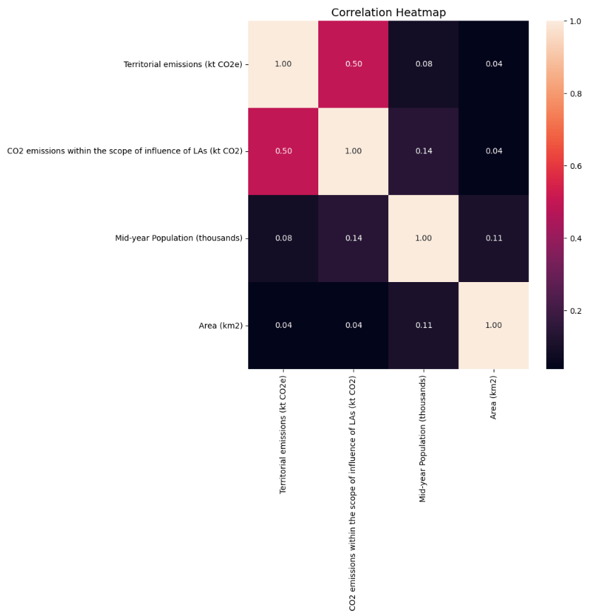
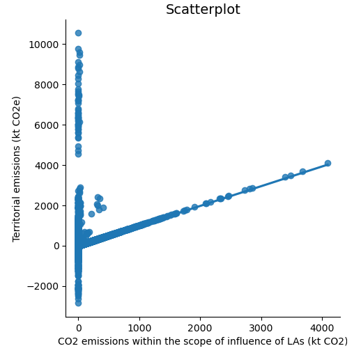
I visualized Territorial emissions (kt CO2e) and CO2 emissions within the scope of influence of LAs (kt CO2) as they had a correlation coefficient of 0.50 which was the largest correlation coefficient between any of the variables. This did not result in a good correlation as approximately half of the data points on the scatterplot follow the trendline, and half do not.

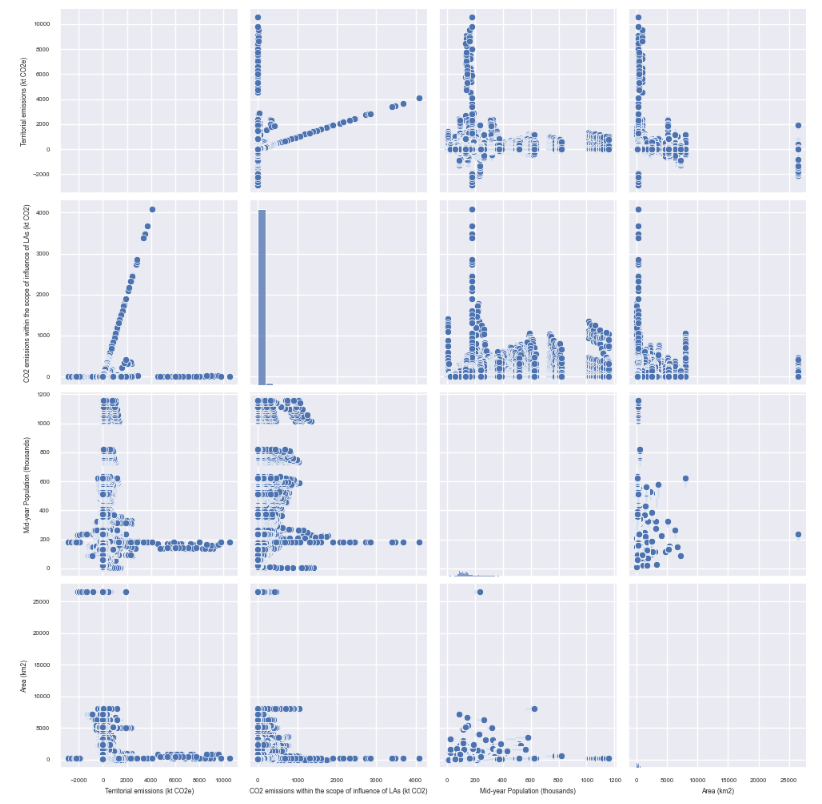
I generated a pair plot to visually see the relationships between all the numeric variables. The visualizations in the pair plot showed potential for further exploration into the relationship between Mid-year Population (thousands) and Area (km2).

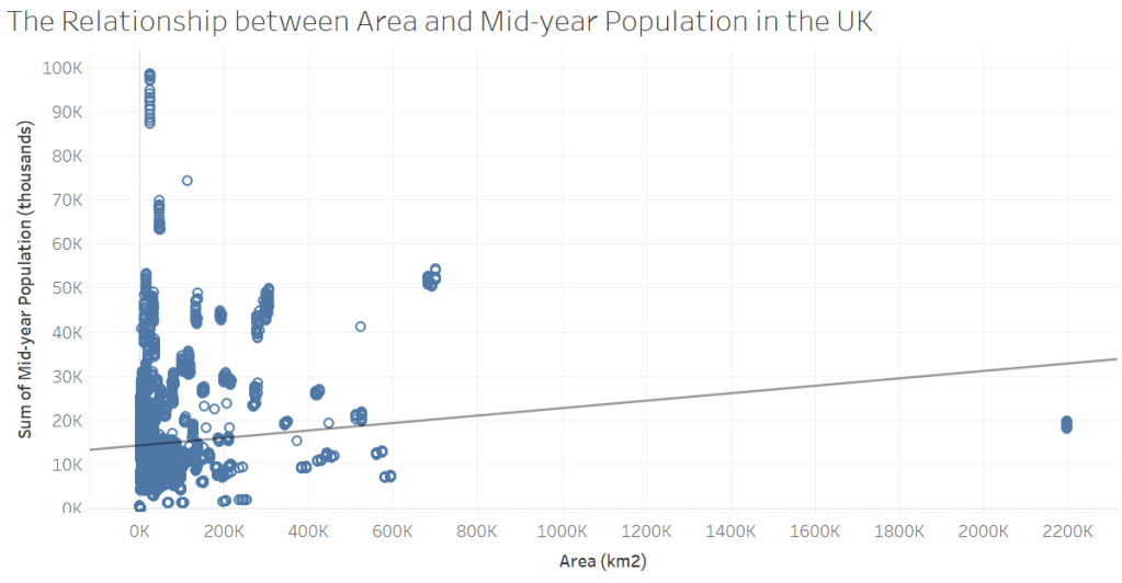
Linear Regression

I hypothesized that as area increases, mid-year population increases. To test my hypothesis, I first used the linear regression machine learning algorithm which involved splitting the dataset into a training set and a test set, creating and fitting a regression object on the training set, and creating a prediction for y on the test set. The linear regression was not a good fit for the data as many data points did not follow the regression line, which indicates that linear regression did not accurately predict the effect of area on mid-year population.

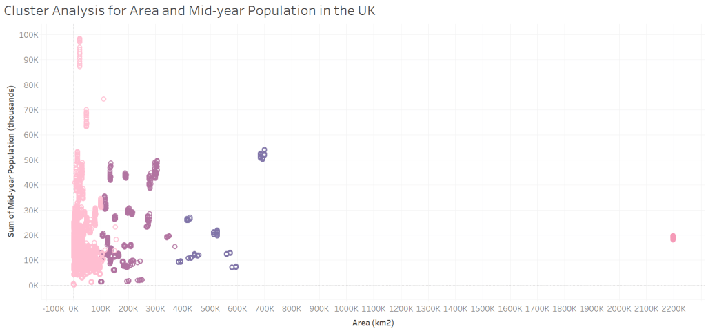
Cluster Analysis

Since the linear regression technique was not adequate for describing the relationship between area and mid-year population, I conducted a cluster analysis which resulted in four clusters. The cluster with the largest area, the pink cluster, has the second-highest mid-year population and highest territorial emissions. The cluster with medium area, the dark purple cluster, has the second-lowest mid-year populations of all the clusters and lower territorial emissions than the pink cluster. The cluster with low area, the purple cluster, has the highest mid-year populations and the second-lowest territorial emissions. The cluster with very low area, the light pink cluster, has the lowest mid-year populations and territorial emissions. The results of the cluster analysis led to the conclusion that mid-year population does not increase as area increases.

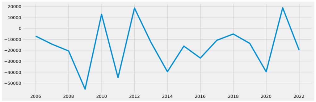
Time-Series Analysis

I conducted a time series analysis to look at the change in territorial emissions overtime from 2005-2022. This required decomposing the time series using an additive model, analyzing the separate time series components, conducting a Dickey-Fuller test to test for stationarity, and then stationarizing the data. I found that territorial emissions have decreased consistently from 2005 to 2022 with three slight increases, once in 2010, once in 2012, and once in 2021. I also found that there is no seasonality in the data along with no unexplained noise. The stationary time series curve:

Challenges

None of the numerical variables in the data set had strong relationships with each other, which made it difficult to obtain insightful results, and consequently, it was difficult to make more specific recommendations for how to reduce greenhouse gas emissions.

Tableau Storyboard

You can access my Tableau Storyboard to see the visualizations generated for this project along with the highlights of the analysis.

Results and Recommendations

Here are the results of the analysis along with recommendations for reducing greenhouse gas emissions:

• Mid-year population does not increase as area increases.
• It is possible that territorial emissions increase as area increases.
• Greenhouse gas emission reduction strategies should be focused on the local authorities within the pink cluster as these represent the areas that have the most emissions.
• The highest priority for greenhouse gas emission reduction strategies should be on local authorities in the pink cluster, followed by the dark purple cluster, purple cluster, and the light pink cluster.

Next Steps

• Analyze Territorial Emissions (ktCO2e) by non-numerical variables such as LA GHG Sub-sector (Local Authority Greenhouse Gas Sub-sector), Greenhouse Gas, and Local Authority.